A Systematic Methodology for the Generation of Lift Passengers under a Poisson Batch Arrival Process

by Dr. Richard Peters, Dr. Lutfi Al-Sharif, Ahmad T. Hammoudeh, Eslam Alniemi and Ahmad Salman

This paper was first presented at the Fifth Symposium on Lift & Escalator Technologies, www.liftsymposium.org.

It is generally accepted that passenger arrivals for lift service follow a Poisson arrival process. Moreover, recent research has also shown that the arrivals take place in batches, rather than single-passenger arrivals. For these reasons, lift traffic simulation software may use the Poisson batch arrival process to generate the time of each batch arrival and the size (number of passengers arriving) of each batch. This provides a better representation of real-life conditions and produces a more realistic simulation. Alternative models for generating passengers for lift traffic-simulation packages are considered. A methodology for generating batch arrival times and the size of each batch is presented.

An important part of any lift traffic simulator is the passenger arrival process. The passenger arrivals represent the demand to which the lift system is subjected. The passenger arrival model should reflect the actual characteristics of the arrival process. This ensures that the output of the simulation is more representative of reality. In this article, alternative arrival models are presented and discussed. A new methodology for generating passenger arrivals is proposed.

Possible Passenger Arrival Generation Models

This section examines possible models with which passengers can be generated for lift traffic simulation. All examples in this section assume a passenger arrival rate (AR), ^λ, of 0.2 passengers per second.

Constant Inter-Arrival Time

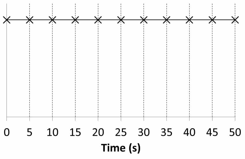
This is a simplification of the passenger arrival process. It is assumed that the time between the arrivals of consecutive passengers is constant (i.e., deterministic rather than random). The time, in seconds, between the arrivals of consecutive passengers or inter-arrival time    can be calculated by:

(Equation 1)

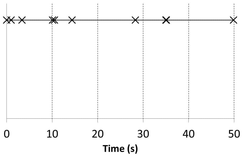
A diagrammatic representation of passenger arrivals against time is shown in Figure 1. As the AR is 0.2 passengers per second, the inter-arrival time is 5 s.

Random Inter-Arrival Time with Uniform Probability Density Function

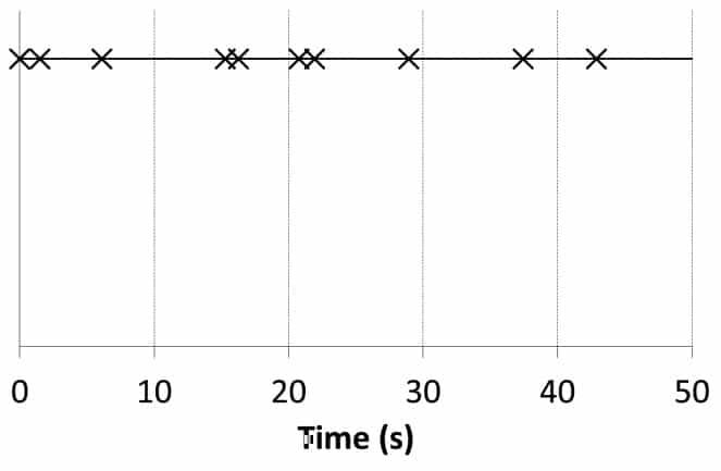
This model assumes that the inter-arrival time is random. However, it contains a simplification of the passenger arrival process by assuming that the distribution of the inter-arrival time is a uniform probability distribution function (PDF). The value of the inter-arrival time has an average value of ^1/λ and varies between 0 s. and twice the average value ^2/λ.

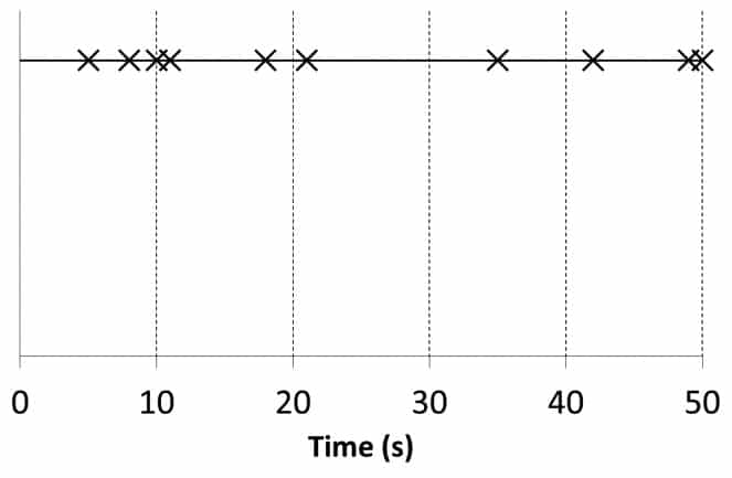
The value of an inter-arrival sample time can be evaluated using Equation 2, where Rand is a function that generates a uniformly distributed random number between 0 and 1. This yields the representation of passenger arrivals given in Figure 2.

   (Equation 2)

Although this model offers a better representation of the passenger arrival process by introducing random passenger arrivals, it assumes that a passenger must arrive in the time period of  ^2/λ, which is not necessarily the case, as a much longer period of time might pass without a passenger arriving. Moreover, the model gives equal probability to all possible values of the inter-arrival time, which is not an accurate reflection of reality.

Random Passenger Arrivals Applying Poisson Probability Density Function

The most widely accepted passenger arrival model is the Poisson process.^{[1, 3 & 4]} This assumes that the number of passengers arriving in a period of time follows a Poisson distribution:

(Equation 3)

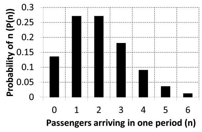
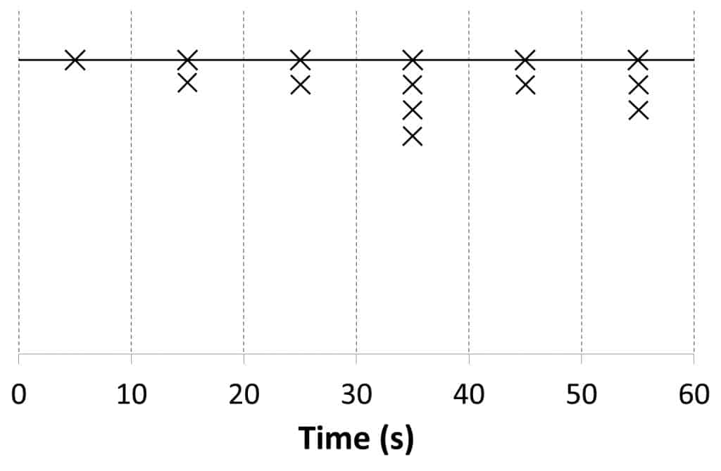
where  P(n) is the probability that the number of passengers arriving in the period of time T is equal to n. The Poisson probability density function has been generated and shown in Figure 3 using the period T of 10 s. Figure 4 shows a representation of passenger arrivals.

The passengers are assumed to arrive in the middle of the period of time T (10 s.), as the actual arrival time of each passenger is not defined. For this reason, this basic application of the Poisson process is unrealistic, even with a smaller T.

A further disadvantage of this approach is that the number of passengers generated in the time period does not necessarily correspond to the AR. This inconsistency between user input and passengers generated can cause confusion to users of traffic-simulation software.

Random Inter-Arrival Time with Exponential Probability Density Function

The random variable in the previous Poisson passenger arrival model is the number of passengers arriving in a time period, T. A better approach is to use the inter-arrival time as the random variable. This can be achieved by considering the time after which one or more passengers are expected, 1 – P (0). Substituting Equation 3 yields Equation 4. Figure 5 shows a representation of passenger arrivals.

(Equation 4)

As for the original Poisson approach, the number of passengers generated in the time period does not necessarily correspond to the AR.

Random Arrival Time in a Given Time Period

To address the inconsistency in passenger numbers, some traffic simulators create the exact number of passengers required by the AR for the time period T. As only whole passengers can be generated, rounding up or down is determined using a random number. Random numbers are used to place the passengers on the time line. This achieves a similar result to the previous model with an exponential probability density function (Figure 6).

A consequence of this approach is that the longer the time period T, the more variation there is in the demand during that period. For example, if T is 5 min., 60 passengers would be generated. If T is 1 hr., 720 passengers would be generated; however, in the first 5 min., there may be 58 passengers, and in the second 5 min., there may be 64 passengers.

Further Considerations

It has been shown that passengers arrive in batches,^[5] also referred to as bulk arrivals.^[2] The probability density function of the batch sizes depends on the nature of the building and time of the day. Thus, for every batch arrival, there are two parameters to generate: the time at which it occurs and the size of the batch.

A Methodology for Generating Passengers for Simulation

Overview

The passenger generation methodology presented in this article combines the most useful features of the methods discussed above: the methodology assumes a random inter-arrival time with exponential probability density function, the total number of passengers is consistent with the expected number of passengers, and the batch size may be building and time specific.

Procedure

For each floor where passengers arrive, consider the total number of passengers generated, p_gen, during the workspace, WS. WS is the time over which passengers are being generated in seconds.  ^λ may be determined from the passenger demand, which, in turn, is calculated according to population and building type.

(Equation 5)

To generate passengers for WS:

1. Calculate the required number of passengers to be generated as shown in Equation 5. Assign the first passenger’s arrival time to 0 s.
2. Using Equation 4, generate the inter-arrival times between all the consecutive passengers.
3. Repeat Step 2 until the number of passengers generated is one more than the required number of passengers, p_gen + 1.
4. Discard the last passenger generated but retain his or her arrival time. This arrival time will be referred to as WS’.
5. It is likely that the value of  WS’ is different from the desired workspace time, WS. Thus, apply a shrink or stretch correction factor, SF = WS/WS’, to the whole set of arrival times. This will ensure that the total passenger generation time is equal to WS.

Example without Batch Arrivals

A building has a population, U, of 1,000 persons and an AR of 12% of the population per 5 min. at the floor being considered. The value of the workspace is 60 s.

(Equation 6)

The expected number of passengers to be generated in the workspace can be calculated as:

 (Equation 7)

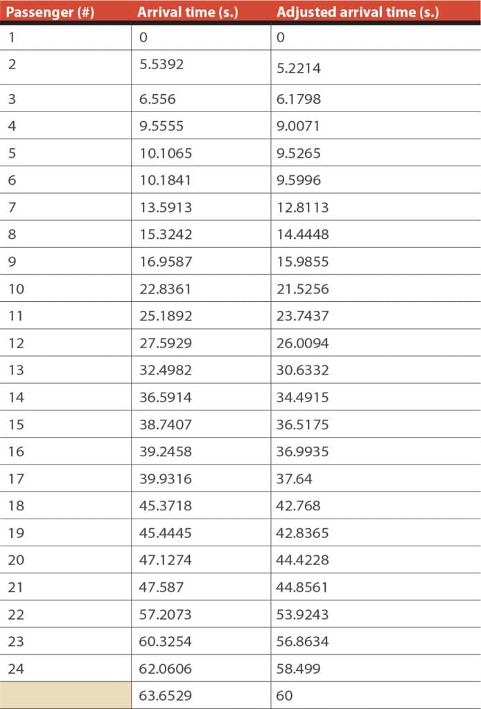
The arrival times of each passenger are shown in Table 1, column 2. As the target number of passengers is 24, the number of passengers initially generated is 25. The 25th passenger will be discarded but his or her arrival time retained. Table 1, column 2 needs to be shrunk or stretched such that exactly 24 passengers arrive within 60 s. The correction factor is found by dividing the desired workspace by the actual workspace.

(Equation 8)

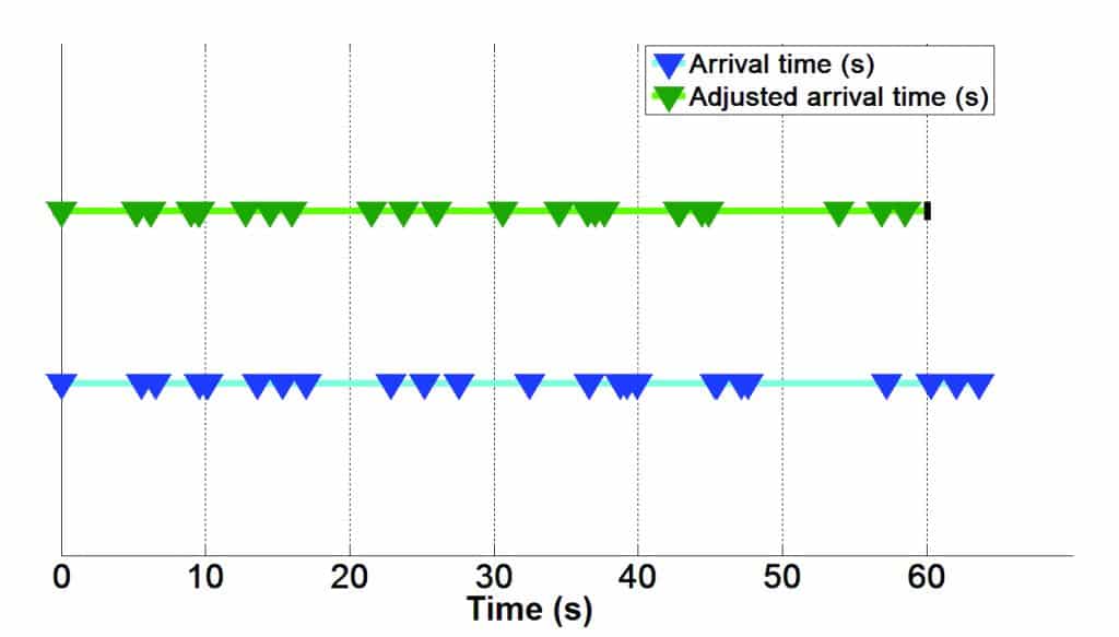
The arrival times are thus adjusted by multiplying them by SF, as shown in Table 1, column 3. The original and adjusted arrival times for the 24 passengers are shown in Figure 7, with each passenger arrival shown as an inverted triangle.

Example with Batch Arrivals

A building has a population, U, of 300 persons and an AR of 4% of the population per 5 min. at the floor is considered here. The value of the workspace is 15 min.

(Equation 9)

Using the value of the AR above, the expected number of passengers to be generated in the workspace can be found as:

(Equation 10)

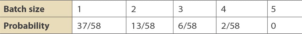
The probability density function that is to be used for the generation of the batch sizes, based on Kuusinen, et al.,[5] is given in Table 2.

The average batch size can be calculated from the PDF as shown below:

(Equation 11)

In order to account for the average batch sizes, calculate the batch AR, λ_b , in batches per second:

(Equation 12)

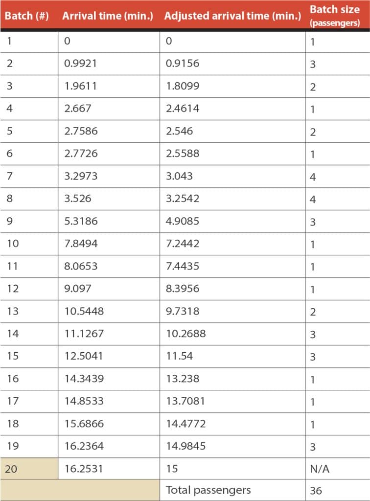
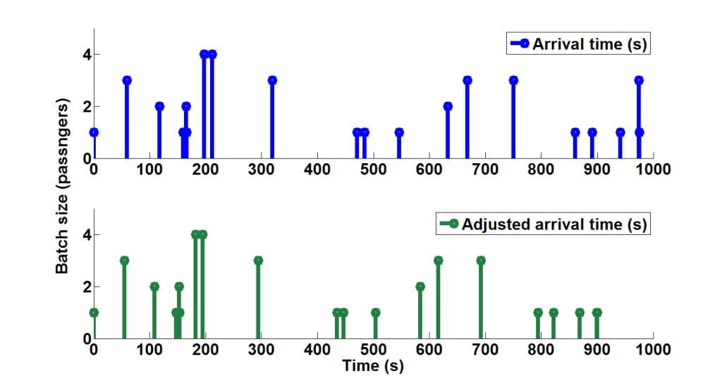
Using the AR for the batches found in Equation 12, the batch arrival times can be generated. These are shown in Table 3 together with the batch sizes. The batch sizes are randomly generated using the batch-size PDF shown in Table 2.

The 20th batch is discarded, but its arrival time is retained. Table 3’s data needs to be shrunk or stretched such that exactly 36 passengers arrive within 15 min. The correction factor is found by dividing the desired workspace by the actual workspace.

(Equation 13)

The arrival times are adjusted by multiplying them by SF as shown in Table 3, column 3. It is worth noting that the initial batch sizes are not changed. The sum of the passengers arriving in 15 min. is 36 passengers, as required.

Conclusions

Alternative models for generating passengers for lift traffic simulation packages have been presented. The first model assumes a constant passenger AR, where the time between passenger arrivals is deterministic and constant. This model is not representative of reality, as it is known that passengers arrive randomly. However, it can be used for the verification of the value of the round-trip time found using calculation. The second model assumes a uniform (rectangular) probability density function, where the inter-arrival time of the passengers randomly varies between 0 and  ^2/λ s. It assumes a passenger must arrive, at most, every  ^2/λ s. and gives equal probability to all values of inter-arrival time between 0 and  ^2/λ s. Neither of these assumptions reflect reality.      

The third model assumes that the number of passengers, n, arriving in a period of time T follows a Poisson process. The passengers are assumed to arrive in the middle of the period of time T, as the actual arrival time of each passenger is not defined. This is unrealistic, even with a smaller T. The fourth model modifies Poisson to allow for exact arrival times to be defined. This is more realistic; however, the random nature of arrivals means that the passengers generated in the time period do not necessarily correspond to the AR.

Another approach creates a Poisson-like arrival process but generates the exact number of passengers expected. Further consideration is given to research that proposes that people arrive in batches. The methodology also shows how to ensure consistency between the actual number of passengers generated in the workspace and the actual number of expected passengers by using a correction factor, SF.

Further Work

A Kolmogorov-Smirnov goodness of fit test has been carried out on real-life survey data to confirm that the model assuming random inter-arrival time with exponential probability density function cannot be rejected. A discussion of determining the destinations of passengers will be provided. Alternative methods of passenger generation will be included in traffic-simulation software, and an assessment on the impact on example designs will be made. This work will be published in future paper(s) and/or article(s). The implication of turnstiles at the entry to the building or lift lobby also needs to be considered.

References
[1] N.A. Alexandris, Statistical Models in Lift Systems, PhD Thesis, University of Manchester, Institute of Science and Technology, 1977.
[2] Norman T.J. Bailey, “On Queueing Processes with Bulk Service,” Journal of the Royal Statistical Society, Series B (Methodological), Vol. 16, No. 1 (1954), p. 80-87.
[3] G.C. Barney, Elevator Traffic Handbook, Taylor & Francis, 2003.
[4] N.A. Alexandris and G.C. Barney, “Three Buildings Surveyed,” University of Manchester Institute of Science and Technology (UMIST), Control Systems Centre report number 350, 1976.
[5] J.M. Kuusinen, J. Sorsa, M.L. Siikonen, and H. Ehtamo, “A Study on the Arrival Process of Lift Passengers in a Multi-Storey Office Building”, BUILDING SERV ENG RES TECHNOL, published online before print November 10, 2011, doi: 10.1177/0143624411427459, November 2012 Vol. 33 No. 4, p. 437-449.