Evaluating Elevator Passenger Average Traveling Time under Incoming Traffic Conditions Using Analytical Formulae and Monte Carlo Method
Jun 1, 2013
by Dr. Lutfi Al-Sharif, Osama F. Abdel Aal and Ahmad M. Abu Alqumsan
Monte Carlo simulation is a powerful tool used in calculating the value of a variable that is dependent on a number of random input variables. For this reason, it can be successfully used when calculating the round-trip time of an elevator, where some of the inputs are random and follow preset probability-distribution functions. The most obvious random inputs are the number of passengers boarding the car in one round trip, their origins (in the case of multiple entrances) and their destinations.
Monte Carlo simulation has been used to evaluate the elevator round-trip time under up-peak traffic conditions. Its main advantage over analytical formula-based methods is that it can deal with all special conditions in a building without the need for evaluating new special formulae. A combination of all of the following special conditions can be dealt with: unequal floor population, unequal floor heights, multiple entrances and top speed not attained in one floor jump. Moreover, this can be done without loss of accuracy by setting the number of runs to the appropriate value.
This paper extends the previous work on Monte Carlo simulation in relation to two aspects: the passenger-arrival-process model and the passenger average traveling time.
The software is developed using MATLAB. The results for the average traveling time are compared to analytical formulae (such as that by So. et al.[4] The results showing the effect of the Poisson arrival process on the value of the elevator round-trip time are also analyzed.
The advantage of this method over analytical methods is again demonstrated by showing how it can deal with the combination of all the special conditions without the loss of accuracy (five conditions if the passenger arrival model is added as Poisson).
The issues of convergence, accuracy and running time are discussed in relation to the practicality of the method.
Introduction
Monte Carlo simulation can be used to evaluate the output value for problems that have a number of random inputs, whereby the probability density functions of the input random variables are known. By generating instances of the random input variable in the form of scenarios and running a large number of scenarios, the expected value of the output of interest can be found by taking the average value of all the scenarios. Scenarios in this paper will be referred to as “trials.”
Monte Carlo simulation has been effectively used to evaluate the round-trip time under up-peak traffic conditions,[1] in finding an optimum parking policy,[2] as well as generating passengers for the purposes of simulating.[3] It offers an advantage over conventional equation-based methods where special conditions exist, such as unequal floor heights, unequal floor populations, top speed not attained in one journey and multiple entrances.
In order to verify the results of the method, an equation is developed to calculate att under up-peak traffic conditions, assuming top speed is attained in one floor journey, a single entrance and equal floor heights. The Monte Carlo simulation results for the att are then compared to the equation developed.[4] The equation is then extended in order to cover the case of unequal floor heights.
Analytical methods for elevator traffic analysis have been extensively covered[5-8] and include the Poisson passenger arrival model,[9-12] the case of the top speed not attained in one floor journey,[13] the case of multiple entrances[14] and discrete time-slice simulation-based methods.[15]
In order to ensure consistency and clarity of the interpretation of the results, the following definitions will be used throughout this paper:
- awt: the average waiting time will be defined as the period from passenger arrival in the lobby until the passenger starts to board the car. Thus, based on this definition, the awt does not include the passenger boarding time.
- att: the average traveling time will be defined as the period from the time the passenger starts to board the car until the passenger has left the car at the destination floor. Thus, based on this definition, the att does include the passenger boarding time. It also includes the passenger alighting time at the destination.
The equation for the att is derived in Derivation of the Equation for the Average Traveling Time. Verification of this equation using the Monte Carlo simulation method is examined in Verification. The equation is then further adjusted for the case of unequal floor heights in Case of Unequal Floor Heights. The effect of the Poisson passenger arrival model is analyzed in The Effect of the Poisson Passenger Arrival Model. A practical elevator-system design example is given in Practical Example. Notes on convergence are presented in Notes on Convergence of the Monte Carlo Simulator. Conclusions are presented in the final section.
Derivation of the Equation for the ATT
An equation for the att has been developed in “New Formula for Estimating Average Travel Time.”[4] The equation derived in this section uses a different approach and is in accordance with the definitions presented earlier.
The approach in deriving the att is to find the expression for each component of the minimum and maximum possible times, and use the average of both.
The att includes four components:
- The boarding and alighting time for the passenger
- The time the passenger spends waiting for other passengers to board and alight
- The time the passenger spends during the elevator stoppage time (where stoppage time includes acceleration and deceleration time, as well as door opening and closing times)
- The time that the passenger spends in the elevator car traveling at top speed
The first component, which is the boarding and alighting time of the passenger, is easy to evaluate:

In order to calculate the second component, it is assumed that on average the passenger will have the remaining P-1 passengers ahead of him/her and the other half behind him/her. Thus, he/she will have to wait for passengers ![]() to board the elevator after he/she has boarded and will have to wait for
to board the elevator after he/she has boarded and will have to wait for ![]() passengers to alight before he/she can alight.
passengers to alight before he/she can alight.

As for the time spent during elevator stops, it is worth noting that all passengers will at least have to wait for the first stop (rational passenger boarding at the ground cannot alight at the ground and must at least wait for the first stop). Thus, all passengers must wait for ts, as a minimum caused by the first stop. As a maximum, a passenger might have to wait for all the S stops above, S.ts. None of the passengers will wait for the last stop (door closing at the highest floor, acceleration and deceleration during the express back journey and doors opening at the main entrance), and hence, the wait is for S stops, rather than S + 1 stops. Taking the average of both values above gives the average time each passenger waits during elevator stops traveling in the up direction:

On average, each stop will traverse a distance of ![]() floors. All passengers will have to wait for that distance to
floors. All passengers will have to wait for that distance to
be traversed at stop speed, at least, as any rational passenger cannot board and leave at the main terminal. As a
maximum, some passengers will have to wait for the whole H floors to be traversed. The minimum time will be
tv . ![]() , while the maximum time will be tv
, while the maximum time will be tv ![]() . S. The following equation takes the average of both times and gives an expression for the time spent during traveling at top speed in the up direction:
. S. The following equation takes the average of both times and gives an expression for the time spent during traveling at top speed in the up direction:

Adding the four terms provides an expression for the att:
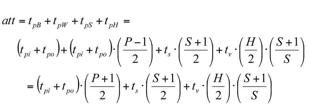
Rearranging and assuming that , the important final result for the att is:

A similar expression for the average traveling time has been derived[4] using a different method and is shown in Equation 7:

It is worth noting that the expression in Equation 6 differs from the one in Equation 7 in that it includes an extra tp, where this accounts for the fact that this definition of waiting time includes passenger boarding time, while Equation 7 excludes passenger boarding time.
It is also worth noting that Equations 6 and 7 implicitly make the following assumptions:
- Top speed is attained in one floor journey.
- Incoming traffic only
- Equal floor heights
- Single entrance
The equation of the round-trip time depends on the values of S (probable number of stops), H (the highest reversal floor) and P (the number of passengers in the car) as shown in Equation 16.

The highest reversal floor is a function of the number of passengers:
H= f (P) (Equation 9)
The probable number of stops is also a function of the number of passengers:
S= f (P) (Equation 10)
The number of passengers in the elevator car is equal to the product of the passenger arrival rate and the actual interval:

But, the interval is in fact a function of the round-trip time, as shown in Equation 12:
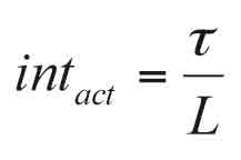
Combining Equations 11 and 12 shows that the number of passengers is a function of the round trip:
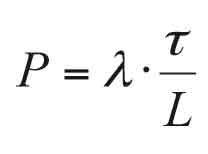
As can be concluded from Equations 8 and 13, the round- trip time is a function of the number of passengers, but the number of passengers is a function of the round-trip time. Thus, the equation for the round-trip time shown in equation (8) is an implicit equation of the round-trip time that can only be solved by the use of an iterative approach (or other mathematical methods such as conformal mapping[11]). This has been addressed as part of a comprehensive design methodology.[17]
When amending the equations for H and S to address the Poisson passenger-arrival model, the term that represents the probability of a passenger not traveling to the ith floor can be amended as shown in Table 1. The probability of a passenger not traveling to floor I, assuming equal floor populations for constant and Poisson arrival modes, is also shown Table 1:
The probability that all the passengers will not go to a floor i is (assuming equal floor populations) for both constant and Poisson arrival models is shown in Table 2:
This can be further developed for the case of unequal floor populations, as shown in Table 3.
The probability of all passengers not going to floor i is equivalent to the probability of the elevator not stopping at floor i. These expressions are used in deriving the values of H and S, as shown in Equations 20-27.
The equation for calculating the average traveling time Equation 8 can cope with a number of special conditions, such as unequal floor heights and Poisson arrival model by using the calculated for the probable number of stops and the highest reversal floor, in accordance with Equations 20-27.
Verification
The derivation of the equation for att has been necessary in order to verify the use of the Monte Carlo simulation. A repeat of the calculations carried out in “New formula for estimating average travel time,”[4] has been carried out, with the results shown in Table 6. The results show excellent agreement with the calculation results.
Table 6: Verification results for att, comparing calculation and Monte Carlo simulation.
| N | P | Analytical equation, assuming constant arrival process (Equation 7) | Monte Carlo simulation (assuming constant arrival process) |
| 10 | 6.4 | 48.19 | 48.18 |
| 10 | 16.8 | 74.46 | 74.40 |
| 13 | 6.4 | 53.65 | 53.67 |
| 13 | 16.8 | 84.00 | 84.00 |
| 16 | 10.4 | 73.27 | 73.27 |
| 16 | 20.8 | 101.97 | 101.97 |
| 20 | 10.4 | 80.70 | 80.72 |
| 20 | 20.8 | 112.85 | 112.85 |
| 23 | 12.8 | 94.74 | 94.65 |
| 23 | 26.4 | 135.00 | 135.03 |
However, the strength of the Monte Carlo simulation method becomes clear when the special conditions exist (such as top speed not attained or multiple entrances), with which the calculation method fails to deal. This will be illustrated later in this article.
Case of Unequal Floor Heights
In the case where the floor heights are unequal, this will have an effect on the calculation of the round-trip time equation. The equation for the round-trip time or att can be amended as follows in order to account for this case.
The effect of the unequal floor heights can be taken into consideration by assuming an effective floor height df eff that can be inserted into the original round-trip-time equation.
The effective floor height df eff is the expected value of the floor height. The effective floor height is the weighted average of all the floor heights, multiplied by the probability of the elevator passing through that floor. In order for the elevator to pass through a floor, it should travel to any of the floors above that floor. Thus, it is necessary to find the probability of the elevator traveling above a certain floor, i.
The probability of the elevator not stopping at a certain floor, assuming equal floor populations is the probability that passenger j will stop at a floor i (assuming equal floor populations and a constant passenger-arrival model).

Thus, the probability that passenger j will not stop at a floor i is:

But, the car contains P passengers. So, the probability that none of them will stop at floor i is the product of all their respective probabilities:

The probability that the lift will not travel any higher than a floor i is the probability that it will not stop on floor i + 1, i + 2 or i + 3 all the way to floor N. This is expressed as the product of these individual conditional probabilities:

This can be re-written as:

Putting all terms inside the same bracket gives:

This simplifies to:

Thus, the probability that the lift will travel above the floor i is:

Thus, the expected value of the travel distance can be calculated as the weighted average of the various floor heights as follows:

The last term above reduces to zero (as it is impossible for the elevator to pass through floor N). The expected floor height is obtained by dividing the expected total travel distance by the highest reversal floor, H. So, the equation for the effective floor height can be expressed as shown in equation (36) (assuming equal floor populations and a constant passenger arrival model):
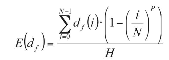
The same procedure can be used to develop the equation for the case of unequal populations and the Poisson passenger-arrival model.
A building with 20 floors above ground was analyzed to illustrate the difference in effective floor height. The floor heights are shown in Table 7. It will be assumed that the floor populations are equal, and that the passenger arrival process is constant (rather than Poisson). It will be also assumed that the number of passengers (P) is 13.
| Floor # | i | df(i) (m) |
| L20 | 21 | 3.2 |
| L19 | 20 | 3.2 |
| L18 | 19 | 3.2 |
| L17 | 18 | 4.2 |
| L16 | 17 | 4.2 |
| L15 | 16 | 4.2 |
| L14 | 15 | 4.2 |
| L13 | 14 | 4.2 |
| L12 | 13 | 4.2 |
| L11 | 12 | 4.2 |
| L10 | 11 | 4.2 |
| L9 | 10 | 4.2 |
| L8 | 9 | 4.2 |
| L7 | 8 | 4.2 |
| L6 | 7 | 4.2 |
| L5 | 6 | 4.2 |
| L4 | 5 | 4.2 |
| L3 | 4 | 6 |
| L2 | 3 | 6 |
| L1 | 2 | 6 |
| G | 1 | 8 |
| N | P | Analytical Equation, assuming constant arrival process (Equation 7) | Monte Carlo Simulation (assuming constant arrival process) | Monte Carlo Simulation (assuming Poisson arrival process) | ||
| att | att | t | att | t | ||
| 10 | 6.4 | 48.19 | 48.18 | 114.26 | 47.37 | 111.72 |
| 10 | 16.8 | 74.46 | 74.40 | 170.82 | 73.90 | 169.49 |
| 13 | 6.4 | 53.65 | 53.67 | 131.27 | 53.08 | 128.83 |
| 13 | 16.8 | 84.00 | 84.00 | 197.40 | 83.36 | 195.75 |
| 16 | 10.4 | 73.27 | 73.27 | 180.98 | 72.60 | 178.80 |
| 16 | 20.8 | 101.97 | 101.97 | 241.80 | 101.25 | 240.21 |

Applying Equation 24 to evaluate the highest reversal floor gives a value for H of 18.95 (assuming floor numbers run from 1-21). Then, applying Equation 36 to evaluate the effective floor height gives a value of 4.62 m. This can be compared to the average floor height of all floors, which is 4.50 m. A difference of 0.12 m exists per floor.
Table 7: The floor heights for a building with 20 floors above ground
The average passenger traveling time can be calculated in order to assess the effect of unequal floor heights, using Equation 7. Using the parameters shown below, whereby the rated speed is attained in one floor journey, only a single entrance and a constant passenger-arrival model is assumed:
- tdo = 2 s.
- tdc = 3 s.
- tsd = 0.5 s.
- tao = 0 s.
- tpi = 1.2 s.
- tpo = 1.2 s.
- v = 1.6 mps
- a = 1 mps2
- j = 1 mps3
The calculation and Monte Carlo simulation results for both round-trip time and att are shown in Table 8.
Using the effective floor height results in a difference of around 3 s. for the round-trip time and a difference of around 1 s. for att. Moreover, the Monte Carlo simulator gives identical results to the calculation method of the amended equation.
The Effect of the Poisson Passenger-Arrival Model
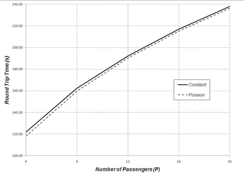
Further investigation regarding the effect of the passenger arrival model on the round-trip time and the att is carried out in this section. Table 9 shows the att and the round-trip time for a number of buildings using the constant passenger-arrival model and the Poisson arrival model. The assumption of a Poisson arrival model results in a small reduction of the values of the round-trip time and the att.
In general, as the number of passengers changes, the Poisson arrival model results in a smaller value of the round-trip and average traveling time, as shown in Figures 1 and 2, respectively.
Practical Example
In order to illustrate the use of the Monte Carlo Simulation method in the elevator traffic design, the following practical example is presented. The example is shown in order to illustrate the use of the method for the combination of the following special cases:
- Constant passenger arrival model
- Unequal floor populations
- Unequal floor heights
- Top speed not attained in one floor journey
- Multiple entrances
An office building has an arrival rate (AR%) of 12%. It is desired to design the elevator system such that a target interval of 30 s. is achieved. The automated design method developed in “Automated Optimal Design Methodology of Elevator Systems using Rules and Graphical Methods (the HARint plane)”[17] is used for the design, and the Monte Carlo simulation is used to calculate the round-trip time, as shown in “The Use of Monte Carlo Simulation in Evaluating the Elevator Round-Trip Time under Up-Peak Traffic Conditions.”[1]
The following parameters are used:
- tdo = 2 s.
- tdc = 3 s.
- tsd = 0.5 s.
- tao = 0 s.
- tpi = 1.2 s.
- tpo = 1.2 s.
- v = 4 mps (top speed will not be attained in one floor journey.[16])
- a = 1 mps2
- j = 1 mps3
The resultant design is shown below:
- Constant passenger arrival model
- Round-trip time: 177.72 s.
- Average traveling time: 71.73 s.
- Number of elevators: seven
- Target interval: 30 s.
- Actual Interval: 25.39 s.
- Actual passenger P: 10.15 passengers
- Car capacity: 13 passengers/1000 kg
- Car loading: 78%
| Floor # | df(i) (m) | Entrance arrival percentage | Population |
| L20 | 4 | – | 30 |
| L19 | 4 | – | 38 |
| L18 | 4 | – | 38 |
| L17 | 4 | – | 38 |
| L16 | 4 | – | 38 |
| L15 | 4 | – | 38 |
| L14 | 4 | – | 38 |
| L13 | 4 | – | 38 |
| L12 | 4 | – | 38 |
| L11 | 4 | – | 38 |
| L10 | 4 | – | 38 |
| L9 | 4 | – | 38 |
| L8 | 4 | – | 38 |
| L7 | 4 | – | 38 |
| L6 | 4 | – | 38 |
| L5 | 4 | – | 38 |
| L4 | 4 | – | 100 |
| L3 | 6 | – | 100 |
| L2 | 6 | – | 100 |
| L1 | 6 | – | 100 |
| G | 8 | 70% | – |
| B1 | 3.2 | 10% | – |
| B2 | 3.2 | 10% | – |
| B3 | 3.2 | 10% | – |
| Number of Trials | ||||||
| 10 | 100 | 1,000 | 10,000 | 100,000 | 1,000000 | |
| Readings for the round-trip time (s.) | 150 | 154.7813 | 153.8286 | 154.1935 | 154.1368 | 154.1514 |
| 153.87 | 153.8205 | 154.3263 | 154.1499 | 154.205 | 154.1547 | |
| 152.745 | 152.9183 | 153.6842 | 153.8559 | 154.1622 | 154.1546 | |
| 155.7375 | 152.6933 | 153.7789 | 153.9662 | 154.1579 | 154.1587 | |
| 154.6125 | 153.4088 | 154.1551 | 154.0913 | 154.1548 | 154.1553 | |
| 156.3 | 155.4473 | 153.8216 | 154.2747 | 154.1166 | 154.1585 | |
| 156.5475 | 154.0455 | 154.0831 | 154.1364 | 154.1485 | 154.1510 | |
| 162.2175 | 153.3323 | 154.5007 | 154.1614 | 154.2053 | 154.1533 | |
| 156.5475 | 153.708 | 154.4249 | 154.1944 | 154.1861 | 154.1614 | |
| 147.75 | 155.049 | 154.2289 | 154.1461 | 154.1513 | 154.1557 |
Notes on Convergence of the Monte Carlo Simulator
In this section, some analysis is carried out on the convergence of the final result from the Monte Carlo simulator as used to calculate the round-trip time and att.
The number of trials can be selected to achieve better accuracy. The round-trip time results for a sample building are shown in Table 11. The analysis is carried out 10 times for each number of trials.
The results of all the Monte Carlo simulations are plotted as a scatter diagram in Figure 3 in order to visually convey the relationship between the accuracy of the method against the number of trials. The effect on accuracy of the final answer against the number of trials is plotted in Figure 4. Based on the results in the figure, 100,000 trials are required for accuracies better than ± 0.1%.
For the example in Figure 4, an analysis is shown of the running time for the increased number of trials and the resultant accuracy. This provides a guide to the designer in terms of trading accuracy with running time.
It is worth noting that these running times are based on the running of MATLAB code. Use of other tools, such as C++, for example, would provide much faster software, significantly reducing the running time.
| Number of iterations | Percentage deviation from the mean | Running time (s.) (for the example of 10 floors above ground, 13 passengers) |
| 10 | ±4.678% | <1 |
| 100 | ±0.895% | <1 |
| 1,000 | ±0.265% | <1 |
| 10,000 | ±0.136% | <1 |
| 100,000 | ±0.029% | 7 |
| 1,000000 | ±0.003% | 70 |
Conclusions
Monte Carlo simulation has been used to calculate the average passenger traveling time in an elevator system under up-peak traffic conditions. The results of the Monte Carlo simulation have been verified for the simplest cases using an analytical formula for the att that has been derived. This verification showed good agreement.
The analytical equation was further developed to deal with the case of unequal floor heights, and further verification was carried out with good agreement. The analytical equations for the att can be applied to the cases of unequal floor populations and Poisson passenger-arrival model.
The strength of the Monte Carlo simulation comes to the fore when the combination of the following special conditions exist in a building: unequal floor heights, unequal floor populations; multiple entrances, Poisson arrival model and top speed not attained. A practical design example is given to show how the method can be used to calculate the round-trip time and att.
Commentary is given on the rate of convergence of the method and the effect of the number of trials on the accuracy of the result. A guide is provided to the designer as to the tradeoff between the number of trials, accuracy of the method and the running time.
Presented at the 1st Symposium on Lift & Escalator Technologies at the University of Northampton, September 2011

Figure 1: Round-trip time for a 16-floor building for both constant and Poison arrival passenger models 
Figure 2: Att for a 16-floor building under constant and Poisson passenger arrival models 
Figure 3: Convergence of the value of the round-trip time as the number of trials is increased 
Figure 4: Deviation percentage of the round-trip time from the mean against the number of trials
References
[1] Lutfi Al-Sharif, Husam M. Aldahiyat and Laith M. Alkurdi, “The Use of Monte Carlo Simulation in Evaluating the Elevator Round Trip Time under Up-peak Traffic Conditions,” Building Services Engineering Research and Technology 0143624411414837, first published on October 21, 2011 as doi:10.1177/0143624411414837.
[2] C. M. Tam and Albert P. C. Chan, “Determining free elevator parking policy using Monte Carlo simulation,” International Journal of Elevator Engineering, Volume 1, 1996, pp. 24-34.
[3] Bruce A. Powell, “The role of computer simulation in the development of a new elevator product,” Proceedings of the 1984 Winter Simulation Conference, pp. 445-450, 1984.
[4] So A.T.P. and Suen W.S.M., “New formula for estimating average travel time,” Elevatori, Volume 31, No. 4, 2002, pp. 66-70.
[5] CIBSE, CIBSE Guide D: Transportation Systems in Buildings, published by the Chartered Institute of Building Services Engineers (CIBSE), Third Edition, 2005.
[6] G.C. Barney, Elevator Traffic Handbook: Theory and Practice, Taylor & Francis, 2002.
[7] R. D. Peters, “Lift Traffic Analysis: Formulae for the General Case,” Building Services Engineering Research and Technology, Volume 11, No. 2, 1990
[8] Richard D. Peters, “The theory and practice of general analysis lift calculations,” Proceedings of the 4th International Conference on Elevator Technologies (Elevcon 1992), Amsterdam, May 1992.
[9] N. A. Alexandris, G. C. Barney, C. J. Harris, “Multi-car Lift System Analysis and Design,” Applied Mathematical Modeling, Volume 3, August 1979.
[10] N. A. Alexandris, G. C. Barney, C. J. Harris, “Derivation of the mean highest reversal floor and expected number of stops in lift systems,” Ap-plied Mathematical Modeling, Volume 3, August 1979.
[11] N. A. Alexandris, C. J. Harris, G. C. Barney, “Evaluation of the handling capacity of multi-car lift systems,” Applied Mathematical Modeling, Volume 5, February 1981.
[12] N. A. Alexandris, “Mean highest reversal floor and expected number of stops in lift-stairs service systems of multi-level buildings,” Applied Mathematical Modeling, Volume 10, April 1986.
[13] N.R. Roschier, M.J., Kaakinen, “New formulae for elevator round trip time calculations,” ELEVATOR WORLD supplement, 1978.
[14] Lutfi Al-Sharif, “The effect of multiple entrances on the elevator round trip time under up-peak traffic,” Mathematical and Computer Modeling, Volume 52, Issues 3-4, August 2010, pp. 545-555.
[15] Richard David Peters, “Vertical Transportation Planning in Buildings,” Ph.D. Thesis, Brunel University, Department of Electrical Engineering, February 1998.
[16] Richard D. Peters, “Ideal Lift Kinematics,” Elevator Technology 6, IAEE Publications, 1995.
[17] Lutfi Al-Sharif, Ahmad M. Abu Alqumsan, Osama F. Abdel Aal, “Automated Optimal Design Methodology of Elevator Systems using Rules and Graphical Methods (the HARint plane),” Published online April 12, 2012, doi: 10.1177/0143624412441615, Building Services Engineering Research Technology, April 12, 2012 0143624412441615.
Get more of Elevator World. Sign up for our free e-newsletter.


