Calculation of Elevator Balance Coefficient Based on Aitken’s Interpolation
Mar 1, 2013

by Huang Shaolun, Luo Zhiqun, Dai Qingyou and Wan Jianru
Balance coefficient is an important parameter for the design, implementation and inspection of traction elevators. It is traditionally illustrated by drawing “Load – Current” inspection data curves in sketch or polygon method, both of which inevitably cause inaccuracy in their numerical result. To solve this problem, this article prospers a method with high accuracy in the approach of Aitken’s interpolation. Additionally, for reducing unnecessary storage space, the compression storage technique in the process of interpolation is analyzed in detail. Finally, the method is verified successfully on the MATLAB GUI platform, and the comparisons with different methods shows it performs effectively in accuracy and reliability.
Introduction
Balance coefficient is a crucial parameter for traction elevators, especially in elevator design. The proper range of balance coefficient from 0.40-0.50 is more effective for balancing the weight of an elevator car (either loaded or unloaded) and its counterweight. A suitable balance coefficient can make the elevator more comfortable, safer and less energy consumptive. In the inspection of a traction elevator, this important parameter is calculated by drawing upward trip and downward trip load-current data by graphing. However, in practice, it is hard to always guarantee the result with low error, due to subjectivity. The polygon method is another way to deal with this problem, but its accuracy is far from satisfactory.
Zhou[1] presented a quadratic regression curve solution, but it performs poorly, because the curve does not pass through all the inspection data points. Consequently, the error of balance coefficient increases. Chang[2] presented another method with Newton’s interpolation. However, it does not take the “Runge phenomenon,” which may cause curve distortion in high-order polynomial interpolation, into consideration. So, it is difficult to keep an accurate and reliable result in any case.
Inspection Data Curve Solution Based on Aitken’s Interpolation
According to the Regulation for Lift Supervisory Inspection and Periodical Inspection – Traction and Positive Drive Lift (TSG T7001-2009) of China put into practice on April 1, 2010, the inspection of balance coefficient has changed. Balance coefficient is suggested to be designed in the range from 0.40-0.50 or to meet the particular requirements. As the car carries 0%, 25%, 40%, 50%, 75%, 100% and 110% of its rated load separately, related motor current should be recorded when the car runs at the same level as the counterweight. Then, the load-current upward and downward trip inspection data curves can be drawn. They have a unique cross point for calculation of the balance-coefficient value.
There are two sets (upward and downward trip) of inspection data, each composing of seven pairs of data. A reliable way to improve the calculation in balance-coefficient accuracy is to seek a scientific approach in generating curves. Hence, a novel method of Aitken’s interpolation is introduced to solve this issue.
Aitken’s Interpolation Scheme
The problem of Aitken’s interpolation is usually stated in the following form: find the polynomial L(x) = Ln(x) of a degree not higher than n, the values of which at points xi (i = 0, 1, 2, . . ., n) coincide with the values of the given function; i.e., L(xi) = yi, where xi represents percentage load and yi represents motor current. Geometrically, this means one has to find an algebraic curve of the form Ln(x) = y = a0xn + a1xn – 1 + . . . + an that passes through the given set of interpolation points Mi (xi, yi) (i = 0, 1, . . ., n).
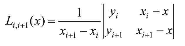
Taking advantage of xi and xi + 1 as interpolation points, here, we can yield the linear-interpolation polynomial Li, i + 1(x) with two initial points:
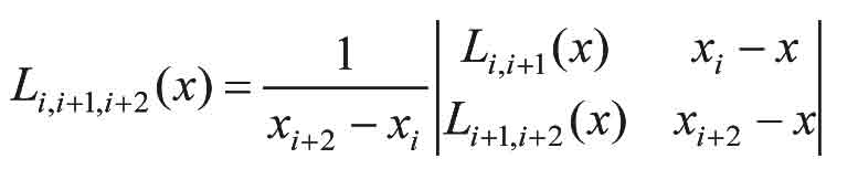
Moreover, considering Li, i + 1(x) and Li + 1, i + 2(x) as two fresh interpolation points, we can obtain the quadratic-interpolation polynomial, which is, utilizing the point xi, xi + 1 and xi + 2:
Therefore, a general polynomial form L0, 1, . . ., n(x) of degree n passing through from interpolation points (x0, y0) to (xn, yn), with all n + 1 interpolation points involved, can be shown as the recursive formula:
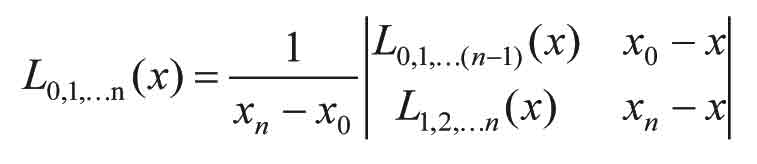
This is the mathematical scheme of Aitken’s interpolation. Formula 3 (the recursive formula) allows one to derive every polynomial from exactly two polynomials of a degree lower by one, which means it is helpful to compute in succession. This recursive formula indicates Aitken’s interpolation is as efficient as Newton’s interpolation on inheritance.
Storage Compression for the Interpolation Process
To simplify computational work, the above findings are usually tabulated. For computing L…(x), it is convenient to use the arrangement of interpolation polynomials in Figure 1. The one located on the principal diagonal with underline is the result of the nth polynomial in the nth step.
In Aitken’s interpolating table, the polynomials in each step are constructed as a lower triangle matrix, which is always stored in memory as a two-dimension array. However, it is important to be aware that when calculating an element in this matrix, it is only related to two elements – one located in the top left corner, and the other on the left side. In other words, all elements are disposable, except those that remain in a diagonal line. Therefore, it is advisable to use one-dimension array technologically for storage compression in the course of Aitken’s computation. The skill is shown in Figure 2, where the elements marked in red fields are updated in each step.
The steps of storage compression in computation are:
- Initiate step counter I = 1. Compute first row in matrix L, then store the results in an array y_temp of one dimension.
- Using ith and jth (j = i + 1, . . ., n) elements in y_temp, interpolation is made by Formula 1 to calculate a fresh result, which then covers the jth element’s location. For example, when i = 1, interpolate with L01(x) and L12(x) for the intended polynomial L012(x), and update this result in the 2nd elements of array y_temp (here, j = i + 1 = 2). Next, compute and successively update the remaining elements L123(x) . . . Ln – 2, n – 1, n(x) in this step.
- Update i = i + 1 and repeat step 2 until it reaches the final polynomial L0, 1, . . . , n(x).
Elevator Data Curves Based on Aitken’s Interpolation
In accordance with the new requirement of TSG T7001-2009, either upward or downward trip curve is inspected strictly at load-current data points. These points are also Aitken interpolation points. If utilizing these seven pairs of points to interpolate directly, a problem may arise: it may be difficult to avoid high-order (up to the sixth order) interpolation polynomials in the solution. In some cases, “Runge phenomena” will appear. An undesirable oscillation will increase computational error and affect computation instabilities. Neither Aitken’s, nor Newton’s interpolation is an exception.
Carefully taking the actual inspection into consideration, it is wise to implement three curves in segmentation, corresponding with Aitken’s interpolation for three groups of data: x0, x1, x2; x2, x3, x4; and x4, x5, x7. This technical improvement not only prevents the final interpolating curves from experiencing Runge phenomena, it also smoothes the entire curve, due to its highest polynomial order being only x2.
Software Design
In order to verify the effectiveness of the proposed method, MATLAB GUI was introduced to be programmed, and several important functions are designed, such as the functions “Aitken’s interpolation with storage compression,” “balance coefficient calculation,” etc. The software flow is shown in Figure 3.
Aitken’s Interpolation with Storage Compression
This function is the main body of Aitken’s interpolation with storage-compression implementation. After a function call, it will return an expression f of its interpolation polynomial, as well as corresponding polynomial coefficients a and the function value y0 (if input) at interpolating point x0.
function [f, a, y0] = interpolation_aitken (x, y, x0)
syms t; syms n;
. . ., . . .
y_temp (1:n) = t;
for(i = 1:n – 1)
for(j = i + 1:n)
y_temp(j) = y(j)*(t – x(i))/(x(j) – x(i)) + y(i)*(t – x(j))/(x(i) –
x(j)); end;
y = y_temp;
simplify(y_temp); end;
simplify(y_temp(n));
f = collect(y_temp(n));
f = vpa(f, 5);
if(nargin==3)
y0 = subs(y_temp(n),’t’,x0);
factors = sym2poly(f); else;
factors(1:n) = y_temp(1:n);
factors = sym2poly(f); end
Aitken’s Interpolation Function
According to the analysis in “Elevator Data Curves Based on Aitken’s Interpolation,” all inspection data points should be segmented into three groups, x(1:3),x(3:5) and x(5:7), to execute interpolation independently:
[f_up1, a_up1]=interpolation_aitken(x(1:3), y1(1:3)); [f_up2, a_up2]=interpolation_aitken(x(3:5), y1(3:5)); [f_up3, a_up3]=interpolation_aitken(x(5:7), y1(5:7)); [f_dowm1, a_dowm1]=interpolation_aitken(x(1:3), y2(1:3)); [f_dowm2, a_dowm2]=interpolation_aitken(x(3:5), y2(3:5)); [f_dowm3, a_dowm3]=interpolation_aitken(x(5:7), y2(5:7));Balance Coefficient Calculation Function
The balance coefficient is the cross point of the upward and downward trip data curves. Called the “balance coefficient,” it can be calculated by finding the difference between these two polynomials algebraically and searching the intersection with the horizontal axis.
flag_solve = 0;
a_delta1 = a_up1 – a_dowm1; r1 = poly2sym(a_delta1);
. . . . . .
if(subs(r2, ‘x’, 40)*subs(r2, ‘x’, 75) < 0)
x0 = fzero(r2, [40 75]);
flag_solve = ‘2’;
elseif(subs(r3, ‘x’, 75)*subs(r3, ‘x’, 110) < 0)
x0 = fzero(r3, [75 110]);
flag_solve = ‘3’;
elseif(subs(r1, ‘x’, 0)*subs(r1, ‘x’, 40)<0)
x0 = fzero(r1, [0 40]);
flag_solve = ‘1’; else;
flag_solve = ‘unsolved’; end;
if(flag_solve~=’unsolved’)
if(flag_solve==’1’)
[temp1, temp2, y0] = interpolation_aitken(x(3:5), y1(1:3), x0); end;
if(flag_solve==’2’)
[temp1, temp2, y0] = interpolation_aitken(x(3:5), y1(3:5), x0); end;if(flag_solve==’3’)
[temp1, temp2, y0] = interpolation_aitken(x(3:5), y1(5:7), x0); end;. . . . . .
end
Application
Software Interface
To verify the feasibility of this method, a software was developed based on MATLAB GUI. Its interface is shown in Figure 4. After updating the “Percentage Load — Motor Current” inspection data, it will output the balance coefficient and the expression of both upward and downward trip data curves.
Comparison
For verifying the advantage of Aitken’s interpolation applied in the elevator balance coefficient, the comparisons were made with the same set of data. Graphs of inspection data curves are shown in Figure 5.
By looking at Figure 5(a), we can easily find the curve isn’t glossy at all. By looking at figure 5(b), we can find the other disappointment – Runge phenomenon at the curve terminal. This also appears in the previous analysis. These two problems will worsen when the real balance coefficient deviates from the range 0.4 to 0.5, reducing the accuracy and reliability of inspection results.
As shown in Figure 5(c), the inspection data curves generated in Aitken’s interpolation method are not only glossy enough, but also devoid of Runge phenomenon. It provides better solution accuracy.
Summary
Balance coefficient is an important parameter for traction elevator design, implementation and inspection. This paper presents a new approach to draw the inspection data curves, which applied Aitken’s interpolation, resulting in high accuracy and reliability. The storage compression in computation was also discussed. The method was realized successfully by MATLAB GUI programming, and the comparisons of curves with different methods showed it performed effectively, both in accuracy and reliability. This software was convenient for inspectors, improving their work efficiency.
Acknowledgment
This research is supported by the General Administration of Quality Supervision Inspection and Quarantine of China – Nonprofit Industry Specialized Research Funding Projects (project number 201310153).
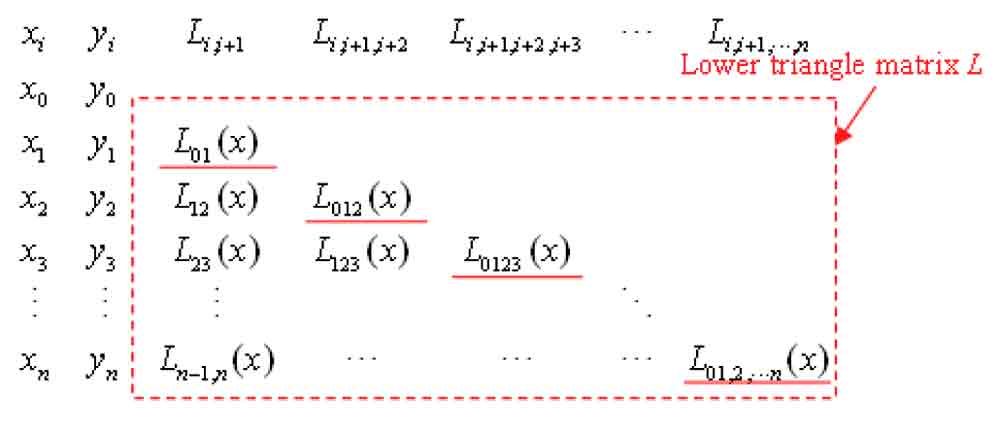
Figure 1: Aitken’s interpolating table 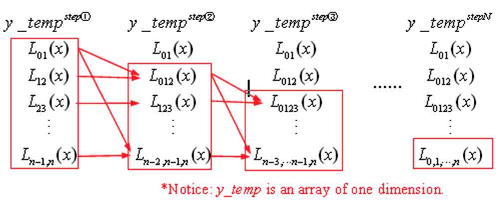
Figure 2: The course of Aitken’s computation with storage compression 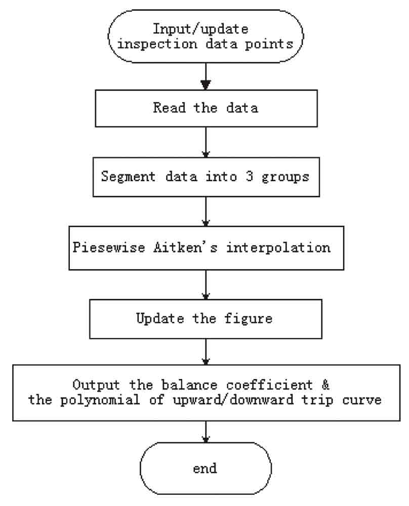
Figur e 3: Software flow 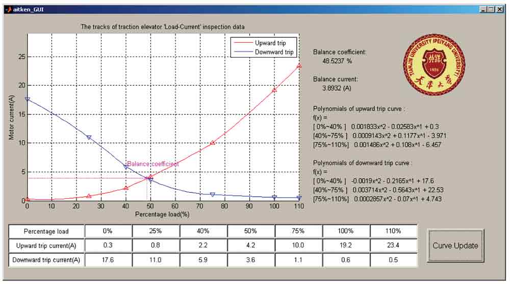
Figure 4: Software interface 
b) Newton’s interpolation method 
(c) Aitken’s interpolation method
References
[1] Runjia Zhou, “Regression Analysis on Elevator Balance Coefficient,” Construction Mechanization, 1989, p. 6.
[2] Zhenyuan Chang, “The Calculation of the Elevator Balance Coefficient with the Software,” China Elevator, 2012, p. 47-49.
[3] Cleve B. Moler, “Numerical Computing with MATLAB,” Society for Industrial & Applied Mathematics, U.S.
[4] D. Kahaner, C. Moler and S. Nash, “Numerical Methods and Software,” Prentice Hall, Englewood Cliffs, New Jersey, 1989.
Get more of Elevator World. Sign up for our free e-newsletter.


